Deep Learning & Computer vision techniques are making progress in every possible field. With growing computing powers many organizations use them to resolve or minimize many day-to-day problems. In a recent talk at AVAR 2018, Quick Heal AI team presented an approach of effectively using Deep Learning for malware classification. Here we are giving detailed technical blog for the same.
Introduction
At the root of most malware attacks lies PE files which essentially causes the resultant damage. A typical attack initiates with the download of a PE file via email, website or other commonly used mechanisms. Traditional methods of detecting such malicious PE files range from rule-based; signature based static methods to behavior-based dynamic methods such as emulators, sandboxes, etc. But they are falling short in the race of generically detecting advanced malware. The figure shown below explains one such example of Crysis Ransomware(Here is the decryption tool for Crysis). Here sample is so obfuscated that it bypasses rule-based or signature-based detection mechanisms easily.
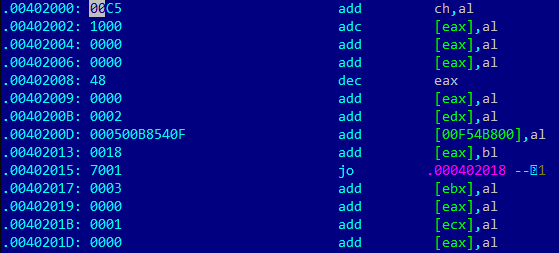
To combat against such mechanisms, we introduced Machine Learning based detection. Where, we use many algorithms like SVM, Random Forest for generic detection.
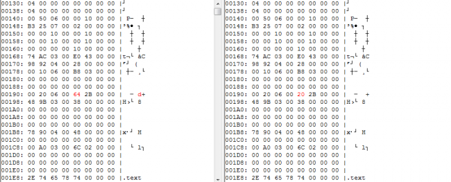
But ML needs sample collection & feature extraction before training. Feature engineering is a tedious task & requires human expertise & time. And it is becoming more complicated day by day as malware are finding ways to bypass it. Techniques like adversarial ML where malware samples are trained to bypass ML are evolving with such a rapid pace to evade property based ML models. Let’s take a look at another example. Here header of XPaj infector sample is shown before and after infection. XPaj makes almost no change in the header of the original file while appending. ML model which are trained on only file header attributes can’t detect these samples.
Deep Learning has come a long way in recently in the field of image classification & computer vision. There are many success stories about image classification problems on Imagenet & Resnet. So we thought about applying image classification to detect malicious files.
Converting PE files into Images
The first challenge is representing PE files in the form of images. Coming from a large set of resources we have a very good amount of PE files in our data set. We label these files as well. To generate images, we used a well-known open source tool called PortEX. This tool mainly generates three types of images as shown in the diagrams below.
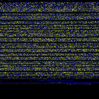
First of them (Fig3) is a byte-plot image, where each byte or a group of bytes represent different color pixel as shown in the figure. And then zeroes are padded at the end to keep the image size constant. In this byte-plot image, zeroes are black and FF by white color pixels. Visible ASCII characters are blue color pixes. And so on.
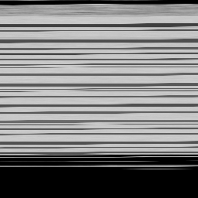
In the second type of images, a scale of the single color pixel represents different bytes. Here (fig 4) bytes are represented by grayscale pixels 0x00 being black and 0xFF white.
In the last type(Fig. 5), PE structure images represent every structure of a PE file in different colored pixels. Like in the example, green represents resources, yellow import, and sky blue pixels represent appended data. After representing PE files into images we can point out the similarities of two different files by simply looking at them. Below are two examples of such files.
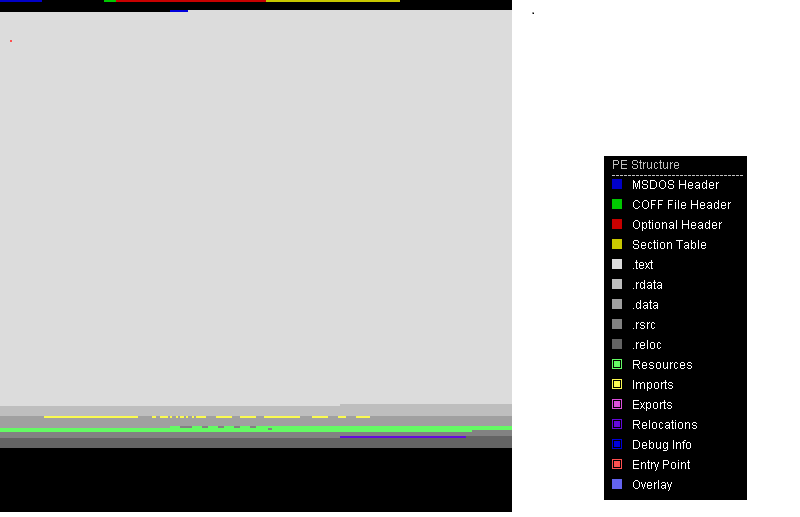
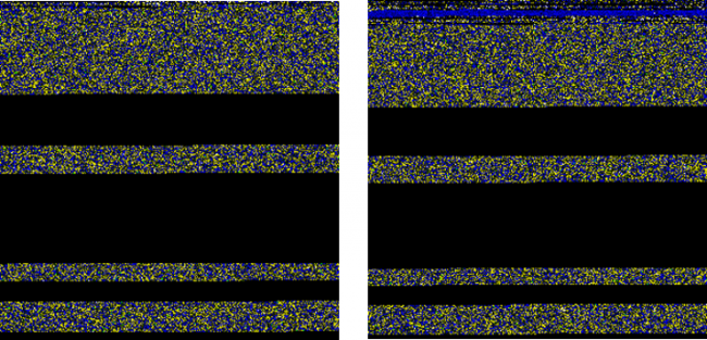
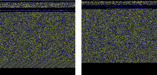
Figure 6 and 7 shows similarities of two different samples of Wannacry and Cerber ransomware respectively.
Deep Learning Overview
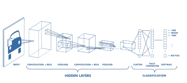
Having a large amount of data i.e. images converted of both clean & malware files, we now apply Deep Learning algorithms on these samples. Deep Learning (DL) or Deep Neural Network (DNN) is a special class of Machine Learning (ML). Artificial Neural Networks (ANN) are building blocks of DNNs. ANNs take inspiration from biological nervous systems. Image classification problems use a special class of DNNs. They are Convolutional Neural Networks (CNN). CNNs are class of simple feed-forward neural network where outputs are passed over the next layers without forming cycles like in the case of recurrent neural networks. They have non-linear activation functions to reduce linearity from trained features. There are four types of layers in CNN and they are
- Convolution Layer
- Pooling Layer
- Flattening Layer
- Fully connected Layer
The Convolution layer uses multiple feature detectors also known as filters or convolution kernels. These filters are slid over an input image to generate feature maps. Each feature detector generates a different feature map corresponding to the feature it is trying to learn. Feature Detectors are small matrices generally of 3X3 dimensions.
Then the pooling layer receives these generated feature maps. This layer is responsible for pooling only those features which are important and leaving behind unwanted features hence reducing over-fitting and improving training time. Pooling can be max pooling, mean pooling, average pooling etc.
Flattening layer basically transforms pooled feature maps into a single column vector. This vector is then passed to a fully connected layer of an ANN. Figure 8 shows all layers of a simple CNN.
Experiments & Results
Once we decided on the algorithm and samples, the training process is similar to all of the Machine Learning methods as we have mentioned in our blog on machine learning. Another useful branch of DL is Transfer Learning. In Transfer Learning a training task uses weights of some another model trained on different training data as initial weights for the training process. Models like VGG16 have good accuracy on Imagenet challenge. We can use them as the starting point of our training. In Table 1 we have shown some of the experiments that we performed using Transfer Learning.
| Model | Model Detail | Detection Ratio | FP Ratio | |||
| Dataset | Architecture | No of Epochs | ||||
| Clean | Malware | |||||
| 1 | 100k | 20k Ransom | VGG16 | 100 | 90.45 | 0.46 |
| 2 | 100k | 20k Ransom | VGG16 last few layer Trainable | 100 | 91.27 | 0.21 |
| 3 | 100k | 50k | VGG16 | 20 | 89.67 | 0.38 |
| 4 | 200K | 100k | VGG16 with layers Trainable | 20 | 91.04 | 0.19 |
(Tab 1: Transfer Learning Experiments)
We got a good detection ratio but False Positive is one of the concerns. As we increased the size of the training set, the results improved further. In the second experiment, we designed multilayered CNN models from scratch. We got good results on a large data set than ransom data. For ransom data, we had a limited number of samples for training (Table 2).
| Model | Model Detail | Detection Ratio | FP Ratio | |||
| Dataset | Architecture | No of Epochs | ||||
| Clean | Malware | |||||
| 1 | 100k | 20k Ransom | 8 Layer CNN Model | 20 | 89.36 | 0.61 |
| 2 | 100k | 50k | 8 Layer CNN Model | 20 | 91.27 | 0.84 |
| 3 | 200K | 100k | 8 Layer CNN Model | 20 | 92.67 | 0.16 |
(Tab. 2: Deep Learning Experiments)
Conclusion
As we are getting good detection ratio with image classification model, Deep learning is going to be a good addition to our arsenal for detecting advanced threats. But as there are false detections too. Therefore, we can’t use it as a stand-alone mechanism. Instead, we are combining the powers of Machine learning, Deep Learning with ever-growing power of Cloud to get great success in detection & will reduce false significantly.

